Machine Learning is a subset of one of the most searched and cryptic term in the computer-world; “Artificial Intelligence” or AI! In machine learning, computers apply statistical learning techniques to automatically identify patterns in data. These techniques can be used to make highly accurate predictions.
To promote learning and adoption, many groups host AI competitions that are targeted at developers. Kaggle is one such platform, known for holding predictive modeling and analytics competitions globally. They frequently analyze and challenge the talented people wanting to excel in ML techniques. As a culture, Synerzip teams frequently take part in these Kaggle competitions to prove their technical competencies.
One such challenge was presented by Mercari. It has Japan’s biggest community-powered shopping app. The challenge was to offer pricing suggestions to sellers. But this is tough as their sellers are able to put just about anything, or any bundle of things, on Mercari’s marketplace.
In this competition, Mercari is challenging people to build an algorithm that automatically suggests the right product prices. Our AI team undertook this real-world Machine Learning challenge.
Challenge:
In this competition, the challenge was to build an algorithm that automatically suggested the right product prices to the sellers. They provided real-world text descriptions of their product as inputted by the user, including details like product category name, brand name, and item condition.
Read more about this challenge here.
Thought Process:
As a strong believer in agile methodology, we divided the problem into few steps. We created small tasks and divided those tasks among team members.
Technology Used:
- Data Exploration and Analysis: Power BI
- Data Processing and Machine Learning: Python
We followed standard machine learning steps as below:
- Understanding the business problem
- Data exploration and analysis using visualizations
- Prepare data using data processing techniques
- Apply machine learning model
- Evaluate model against given train and test data
Normal workflow of any ML Project as shown by Microsoft:Exploratory Data Analysis
Analyzing the given data is a very crucial step in Machine Learning as it provides the context needed to develop an appropriate model for the problem.
With experience, we realized that while doing a time estimation to solve a machine learning problem, a significant part of our time should be spent on data analysis.
There are a number of visualization tools and libraries in R/Python for data analysis. We choose Microsoft Power BI for Exploratory Data Analysis as it is a plug-and-play kind of interactive visualization tool, easy to understand and use.
Data Provided:
Two files were provided for this challenge:
- Train.tsv
- Test.tsv
The files consisted of a list of product listings. These files were tab-delimited.
- train_id or test_id – ID of the listing.
- name – The title of the listing.
- item_condition_id – The condition of the items provided by the seller
- category_name – Category of the listing
- brand_name – Name of the brand
- shipping – 1 if shipping fee is paid by seller and 0 if paid by buyer
- item_description – Full description of the item
Input data for Data Analysis was given in Train.csv.
As we were analyzing the Train.csv, we developed the following few visualizations to analyze the Train data:
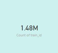
- Record count
To count the total number of records present in Train.csv
- Identify predictor variable
We needed to identify the predictor variable. “Price field” present in Train.csv was the predictor variable.We had to predict prices for items in Test.csv data. Following is a snapshot of Train Data: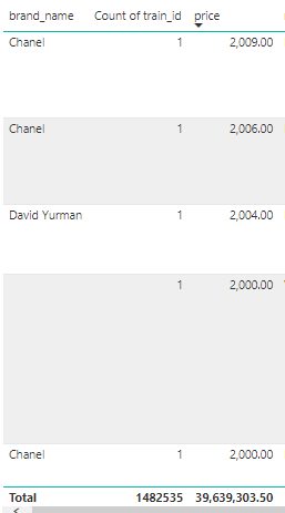
- Count of Train_id by price
As shown in image below, the price range is from 0 $ to around 2000 $. It meant there was some dirty data of 0 $.
- Count train_id by brand_name
As we see in the image below, almost 0.6 million records did not have any brand_names
Data Preprocessing:
The data-mining technique of transforming raw data into an understandable format is called Data preprocessing.
Real-world data is often noisy, inconsistent and/or lacking in certain behaviors and is also likely to contain errors. Data preprocessing is a proven method of resolving such issues. We used the following techniques in data preprocessing-
- Data Cleaning
- Feature Engineering
- Data Transformation
- Data Cleaning:
In Data cleaning, we cleaned the data by deleting records with “0” $ price and filled blank “category_name” values with value as ‘Other’.
- Feature Engineering:
Feature engineering is the process of using domain knowledge of the data to create features that make machine learning algorithms work.
As per data analysis, we added below fields :
- Name + brand_name
We observed most of the brand names also appeared in the Name column. To fill 0.6 million empty brand_name values present in Train.csv, as seen in the chart at point 4, we concatenated Brand_name with name
- Text = Item_description + name + Category_name
Combining the above three fields gives information about the product at one place. After applying IDF (Inverse Document Frequency) this new feature improves the accuracy of the model.
- Category_Name_X = Category_name + Item_condition_id
As per the analysis, Category_name and Item_condition_id have a relationship and so after combining these two fields, the model gives good results.
- Feature Transformation:
- Data Standardization: In Train data, we could see the price was not normally distributed. So we applied logarithmic scaling method to scale down the price in 0.5 – 4 range.
- Data Cleaning:
-
- Dummy Variables: In regression analysis, a dummy variable is a numerical variable used to represent subgroups of the sample in your study. In situations when you want to work with categorical variables which have no quantifiable relationship with each other, dummy variables are used.
Using “LabelBinarizer” we can create dummy variables, so we used” LabelBinarizer” for following fields :
- brand_name
- shipping
- item_condition_id
- Category_name_X
For below categorical variables we used “HashingVectorizer”:
- name
- text
It turns a collection of text documents into a scipy.sparse matrix holding token occurrence counts (or binary occurrence information), possibly normalized as token frequencies if norm=’l1’ or projected on the Euclidean unit sphere if norm=’l2’.
We used a couple of NLP techniques in “HashingVectorizer” to remove unnecessary features and build new features from existing word sequences.
Ngram:
Trigram range to build features ngram_range=(1, 3)
Stopwords:
Stopwords are the words we want to filter out before training the classifier. These are usually high-frequency words that aren’t giving any additional information to our labeling. We supplied custom stopword list : [‘the‘, ‘a‘, ‘an‘, ‘is‘, ‘it‘, ‘this‘, ]
Token Pattern:
Pattern matching is the checking and locating of specific sequences of data of some pattern among raw data or a sequence of tokens.
We used Token Pattern as token_pattern=’\w+‘
It means ‘\w+’ matches any word character (equal to [a-zA-Z0-9_])
Drop very low and very high-frequency features:
In this use case, we observed features having a frequency less than 3 have no significance.
Also features appearing in 90% of records do not have any significance, so we dropped such features.
Tf-idf Transformer:
A Term Frequency is a number of times a word occurs in a given document. The Inverse Document Frequency is the number of times a word occurs in a corpus of documents.
Use of “tf-idf” is to weight words according to how important they are. To have the same scaling and to improve accuracy we concatenated all features and applied Tf-idf to it.
Applying Machine Learning Model
The choice of machine learning algorithm is dependent on the available data and the proposed task at hand. As here we had to predict the price of a product, it was a Regression issue.
Initially, we applied Linear Regression, but as the time limit for the challenge was 60 minutes only and we had 60 million features to cater to, Linear Regression took too much time.
We observed that on Train data, the accuracy was more than Test data and so the model was overfitting.
The number of features was 60 million and the model was overfitting so we decided to apply Ridge Regression.
Ridge Regression penalizes the magnitude of coefficients of the features along with minimizing the error between predicted and actual observations.
Ridge Regression –- Performs L2 regularization, i.e. adds penalty equivalent to the square of the magnitude of coefficients
- Minimization objective = LS Obj + α * (sum of square of coefficients)
Ridge regression performance was much better than Linear regression and we also got good accuracy with it. Here is the Ridge Model we used :
Ridge(solver=’auto’, fit_intercept=True, alpha=0.6, max_iter=50, normalize=False, tol=0.01)
Results
The Synerzip team gave impressive results with good timing:
| Synerzip Kaggle RMSLE (Root Mean Square Logarithmic Error) | 0.4191 |
| Synerzip Kaggle Rank | 79 / 2384 |
| Rank 1 RMSLE on Kaggle | 0.3775 |
| Time Required to complete | 20 Minutes |
| Synerzip Team | Gaurav Gupta, Girish Deshmukh, Nitin Solanki |