A step-by-step guide to performing additive and multiplicative decomposition
Last time, we talked about the main patterns found in time-series data. We saw that trend, season, and cycle are the most common variations in data recorded through time. However, each of these patterns might affect the time series in different ways. In fact, when choosing a forecasting model, after identifying patterns like trend and season, we need to understand how each one behaves in the series. With this goal in mind, let’s explore two different pre-processing techniques — additive and multiplicative decomposition.
Introduction
Classic forecasting methods like ETS and ARIMA have been around for quite some time, but they lacked scalability for larger datasets with more complex temporal patterns. However, the advent of deep learning brought some new light to forecasting. The fact that time-series data has never been more available is a major factor. One example of a deep learning framework for time series forecasting is an open-source solution from Meta, NeuralProphet, which aims at improving Prophet, a tool that performs automated forecasts, by supporting local context. Although NeuralProphet is in beta stage, it already shows promising results. Moreover, there are also implementations that use Long Short-Term Memory (LSTMs) Networks for this type of task.
Despite those advances, time series forecasting is not an easy problem.
In this piece, we focus on ways of further exploring time series data. Our goal is to understand how the various components of a time series behave.
In the end, we hope that such insights will help us with one of the most critical steps in the machine learning pipeline — model selection.
Indeed, choosing an appropriate forecasting method is one of the most important decisions an analyst has to make. While experienced data scientists can extract useful intuitions only by looking at a time series plot, time series decomposition is one of the best ways to understand how a time series behaves.
Time Series Data
Just to recap, time-series data usually exhibit different kinds of patterns. The most common ones are:
- Trend
- Cycles
- Seasonality
Depending on the method we choose, we can apply each one of these components differently. A good way to get a feel of how each of these patterns behaves is to break the time series into many distinct components. Each component represents specific patterns, like trend, cycle, and seasonality.
Let’s begin with classical decomposition methods.
We start off by loading the international airline passengers' time series dataset. This contains 144 monthly observations from 1949 to 1960.
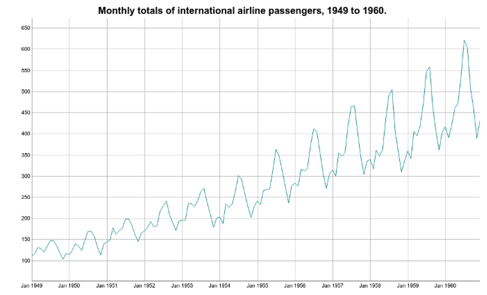
Let’s use this as an example and perform two types of decomposition: additive and multiplicative decomposition.
Before we begin, a simple additive decomposition assumes that a time series is composed of three additive terms.

Likewise, a multiplicative decomposition assumes the terms are combined through multiplication.

Here:
- S represents the Seasonal variation
- T encodes Trend plus Cycle
- R describes the Residual or the Error component.
Let’s explore additive and multiplicative decomposition, step by step.
Additive Decomposition
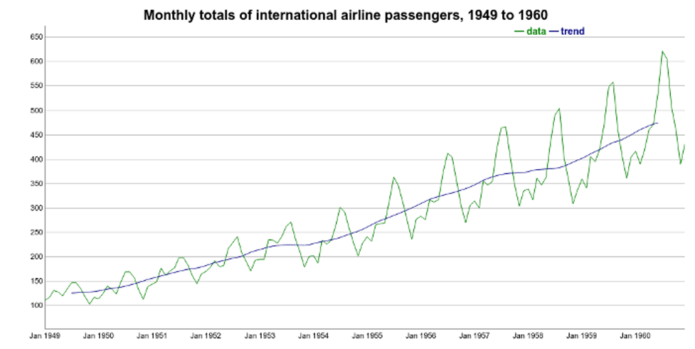
The first step is to extract the trend component of the international airline passenger time series. There are many ways to do this. Here, we compute it as the centered moving average of the data. The moving average smoother averages the nearest N periods of each observation.
Using R, we can use the ma() function from the forecast package. One important tip is to define the order parameter equal to the frequency of the time series. In this case, frequency is 12 because the time series contains monthly data.
We can see the trend over the original time series below:
Once we have the trend component, we can use it to remove the trend variations from the original data. In other words, we can DeTrend the time series by subtracting the Trend component from it.

If we plot the detrended time series, we are going to see a very interesting pattern. The detrended data emphasizes the seasonal variations of the time series.
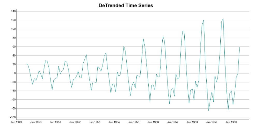
We can see that seasonality occurs regularly. Moreover, its magnitude increases over time. Just keep that in mind for the moment.
The next step is to extract the seasonal component of the data. The approach here is to average the monthly DeTrended data for every year. This can be seen more easily in a seasonality plot.
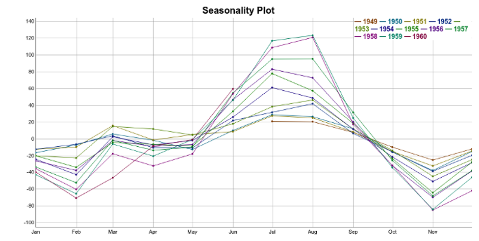
Each line in the seasonality plot corresponds to a year of data (12 data points). Each vertical line groups data points by their frequency. In this case, the x-axis groups data points for each specific month. For instance, for our dataset, the seasonal component for February is the average of all the detrended February values in the time series.
So, a simple way to extract the seasonality is to average the data points for each month. You can see the result in this plot:
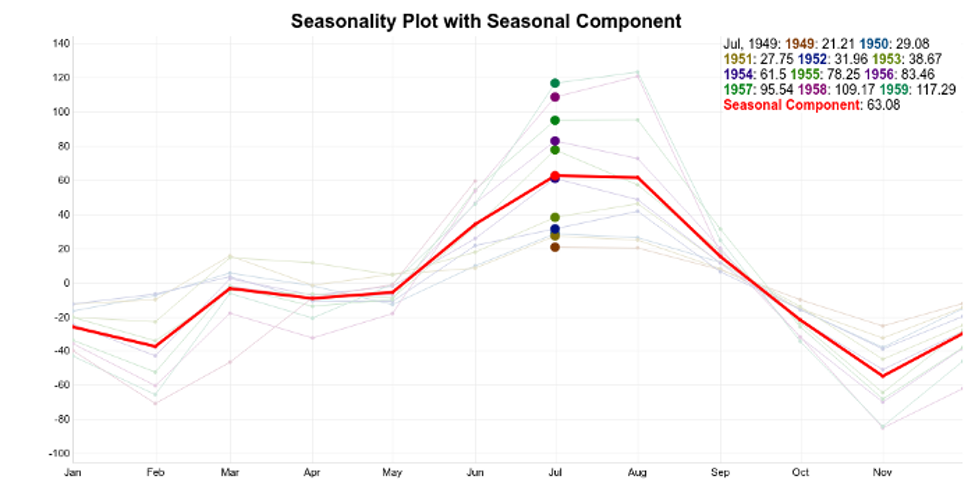
The seasonality component is in red. The idea is to use this pattern repeatedly to explain the seasonal variations on the time series.
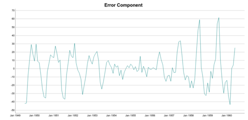
Ideally, trend and seasonality should capture most of the patterns in the time series. Hence, the residuals represent what’s left from the time series, after trend and seasonal have been removed from the original signal.

Of course, we want the residuals to be as small as possible.
Finally, we can put it all together in a seasonality plot:
Now, let’s try to reconstruct the time series using the trend and seasonal components:
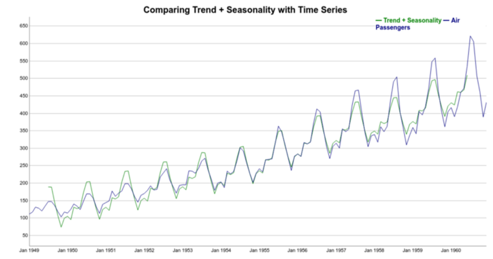
Note that the reconstructed signal (trend+seasonality) follows the increasing pattern of the data. However, it’s clear that in this case the seasonal variations are not well represented. There’s a discrepancy between the reconstructed and original time series. Note that Trend + Seasonality variations are too wide at the beginning of the series but not wide enough towards the end of the series.
That is because additive decomposition assumes seasonal patterns as periodic. In other words, the seasonal patterns have the same magnitude every year and they add to the trend.
But if we take a look again at the detrend time series plot, we see that it’s not true. More specifically, the seasonal variations increase in magnitude over the years. In other words the number of passengers increased, year after year.
Let’s now explore a multiplicative decomposition.
Multiplicative Decomposition
For multiplicative decomposition, the trend does not change. It’s still the centered moving average of the data. However, to detrend the time series, instead of subtracting the trend from the time series, we divide it:

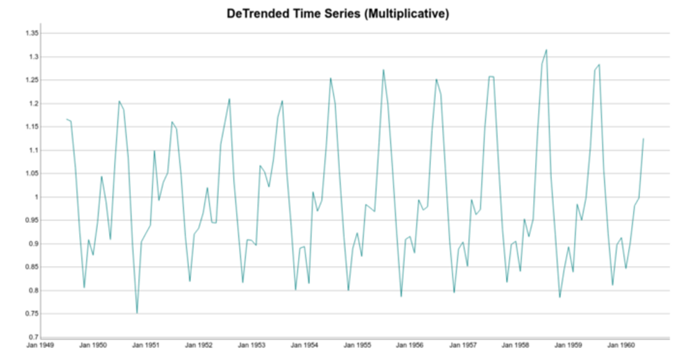
Note the difference between the detrended data for additive and multiplicative methods. For additive decomposition, the detrended data is centered at zero. That’s because adding zero makes no change to the trend.
On the other hand, for the multiplicative case, the detrended data is centered at one. That follows because multiplying the trend by one has no effect either.
Following similar reasoning, we can find seasonal and error components:

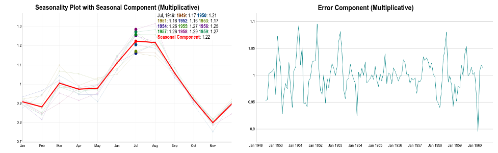
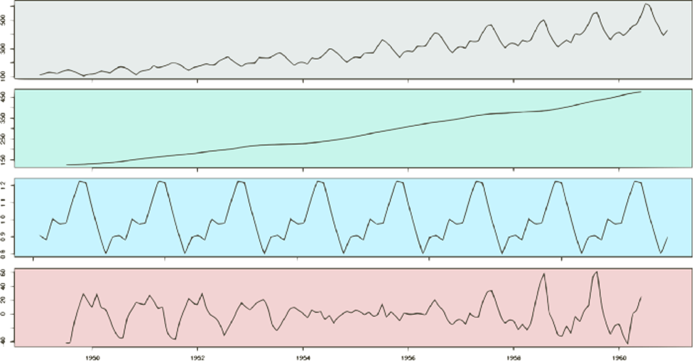
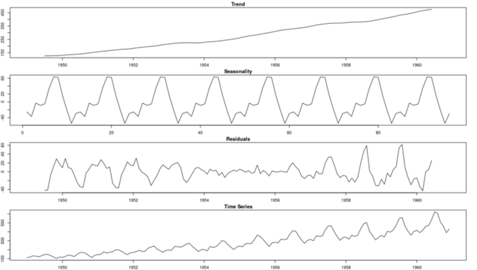
Take a look at the complete multiplicative decomposition plot below. Since it is a multiplicative model, note that seasonality and residuals are both centered at one (instead of zero).
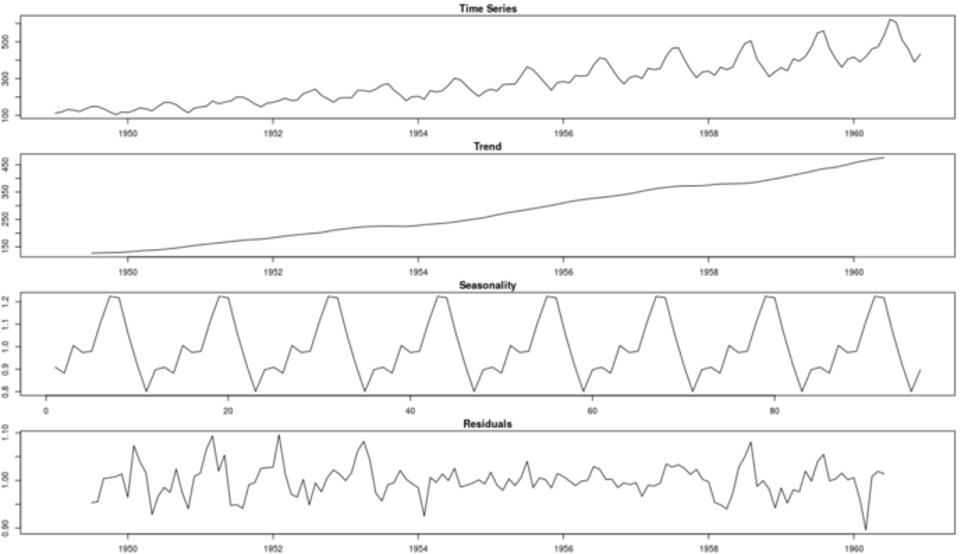
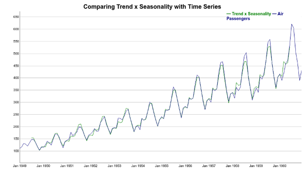
Finally, we can try to reconstruct the time series using the Trend and Seasonal components. It’s clear how the multiplicative model better explains the variations of the original time series. Here, instead of thinking of the seasonal component as adding to the trend, the seasonal component multiplies the trend.
Note how the seasonal swings follow the ups and downs of the original series. Also, if we compare additive and multiplicative residuals, we can see that the later is much smaller. As a result, a multiplicative model (Trend x Seasonality) fits the original data much more closely.
Caveats and Conclusion
It is important to note that simple decomposition methods have some drawbacks. Here, I highlight two of them.
First, using a moving average to estimate the trend+cycle component has some disadvantages. Specifically, this method creates missing values for the first few and last values of the series. For monthly data (frequency equal 12), we will not have estimates for the first and last six months. That is depicted on the Trend figure above.
The estimation of the seasonal pattern is assumed to repeat every year. This can be a problem for longer series where the patterns might change. You can see this assumption on both decomposition plots. Note how the additive and multiplicative seasonal patterns repeat over time.
There are more robust methods like Seasonal and Trend decomposition using Loess — STL — that addresses some of these problems. In a future article, we will talk about STL decomposition and how to use it to build an Exponential Smoothing forecasting method.
Acknowledgment
This article is a contribution of many Encora professionals: Thalles Silva, Bruno Schionato, Diego Domingos, Fernando Moraes, Gustavo Rozato, Isac Souza, Marcelo Mergulhão and Marciano Nardi.
About Encora
Fast-growing tech companies partner with Encora to outsource product development and drive growth. Contact us to learn more about our software engineering capabilities.